Data Preparation and Quality Assessment in Genome Assembly

This workshop provides a hands-on introduction to data preparation, genome assembly, and quality assessment. Participants will explore different assembly approaches and techniques for evaluating the accuracy and completeness of genome assemblies, helping attendees understand key metrics and statistical methods used to assess the quality of genomic data.

Tutorial Setup Instructions

Steps to prepare for the tutorial session:

• Login to Ceres Open OnDemand. For more information on login procedures for web-based SCINet access, see the SCINet access user guide.
• Open a command-line session by clicking on “Clusters” -> “Ceres Shell Access” on the top menu. This will open a new tab with a command-line session on Ceres’ login node.

• Request resources on a compute node by running the following command.

  srun --reservation=wk2_workshop -A scinet_workshop2 -t 05:00:00 -N 1 –c 8  --pty bash   
  

  • For those accessing post-workshop: Remove --reservation=wk2_workshop and change -A scinet_workshop2 to your own project account. For additional information, see our SLURM guide.

• Create a workshop working directory by running the following commands. Note: you do not have to edit the commands with your username as it will be determined by the $USER variable.

  mkdir -p /90daydata/shared/$USER/genome_assembly 
  cd /90daydata/shared/$USER/genome_assembly 
  cp -r /project/scinet_workshop2/Bioinformatics_series/wk2_workshop/day1/ .  
  

Data Preparation

by Viswanathan Satheesh and Sivanandan Chudalayandi

We have two data directories: 01_Data and 02_References

We start with checking the quality of data (Illumina and PacBio HiFi reads)

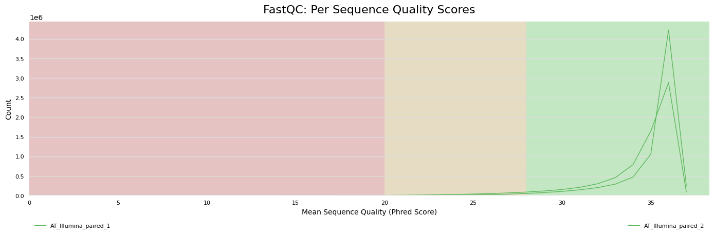
Illumina - FastQC

module load fastqc
mkdir 03_IlluminaQC 
fastqc -o 03_IlluminaQC -t 2 01_Data/AT_Illumina_paired_*gz 

Estimated Time: 1m 8s

• Per base sequence quality

• Per base sequence content

• Overrepresented sequences

• Adapter content

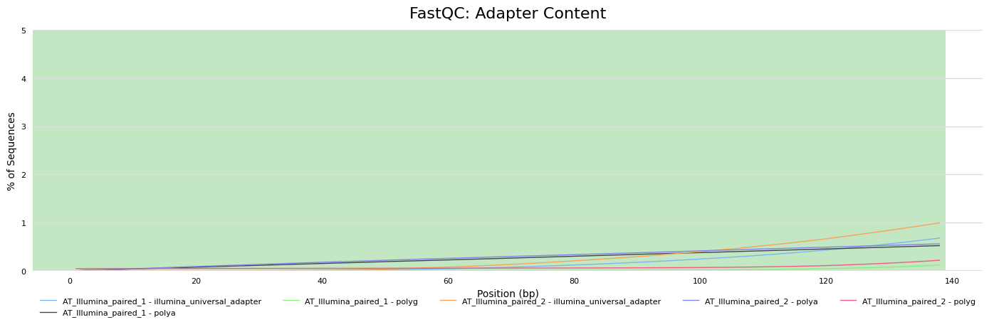
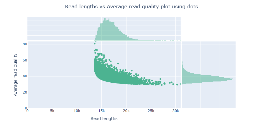
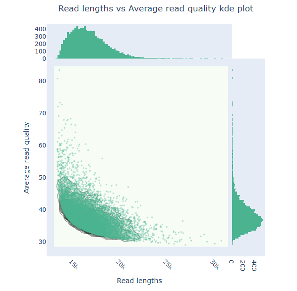
PacBio HiFi - nanoplot

module purge 
module load miniconda 
source activate /project/scinet_workshop2/Bioinformatics_series/nanoplot_conda/NP/ 
mkdir 04_NanoPlotQC 
time NanoPlot --fastq 01_Data/mapped_reads.chr2.filtlong.fastq.gz -o 04_NanoPlotQC --threads 8 

Estimated Time: 2m 17s

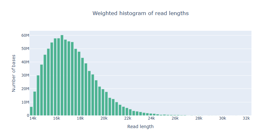
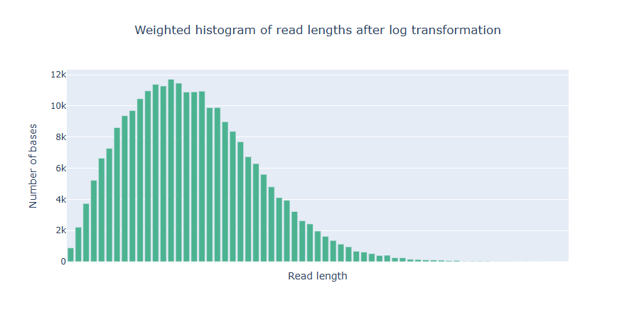
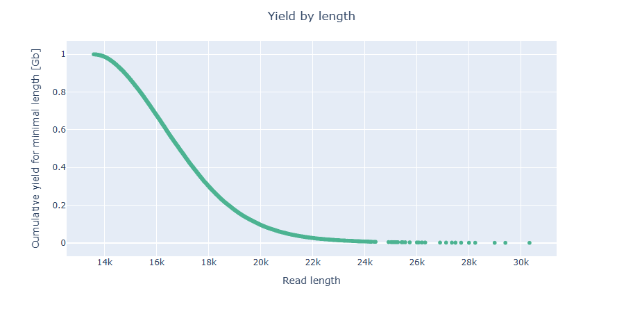
NanoPlot takes about 2 minute and 17 seconds to run.

View Report

Predicting the genome size with Illumina reads with GenomeScope

module purge 
module use /software/el9/spack/lmod/Core 
module load jellyfish 
mkdir 05_GenomeScope 
unpigz 01_Data/AT*gz 

time jellyfish count -m 21 -s 100M -t8 \  
  -C 01_Data/AT_Illumina_paired_* \ 
  -o 05_GenomeScope/reads.jf 

• -m 21: 21-mers
• -s 10M: 10 million reads - this is the number of reads used to estimate the size of the genome
• -t 8: 8 threads

Takes about 1m 50 seconds to run.

time jellyfish histo -t 8 05_GenomeScope/reads.jf > 05_GenomeScope/reads.histo 

• jellyfish histo is used to estimate the size of the genome using the reads.jf file. It outputs the size of the genome in the reads.histo file.

Takes about 20 seconds to run.

We can now copy the reads.histo to our local computer and upload it to GenomeScope

Interpretation of the images:

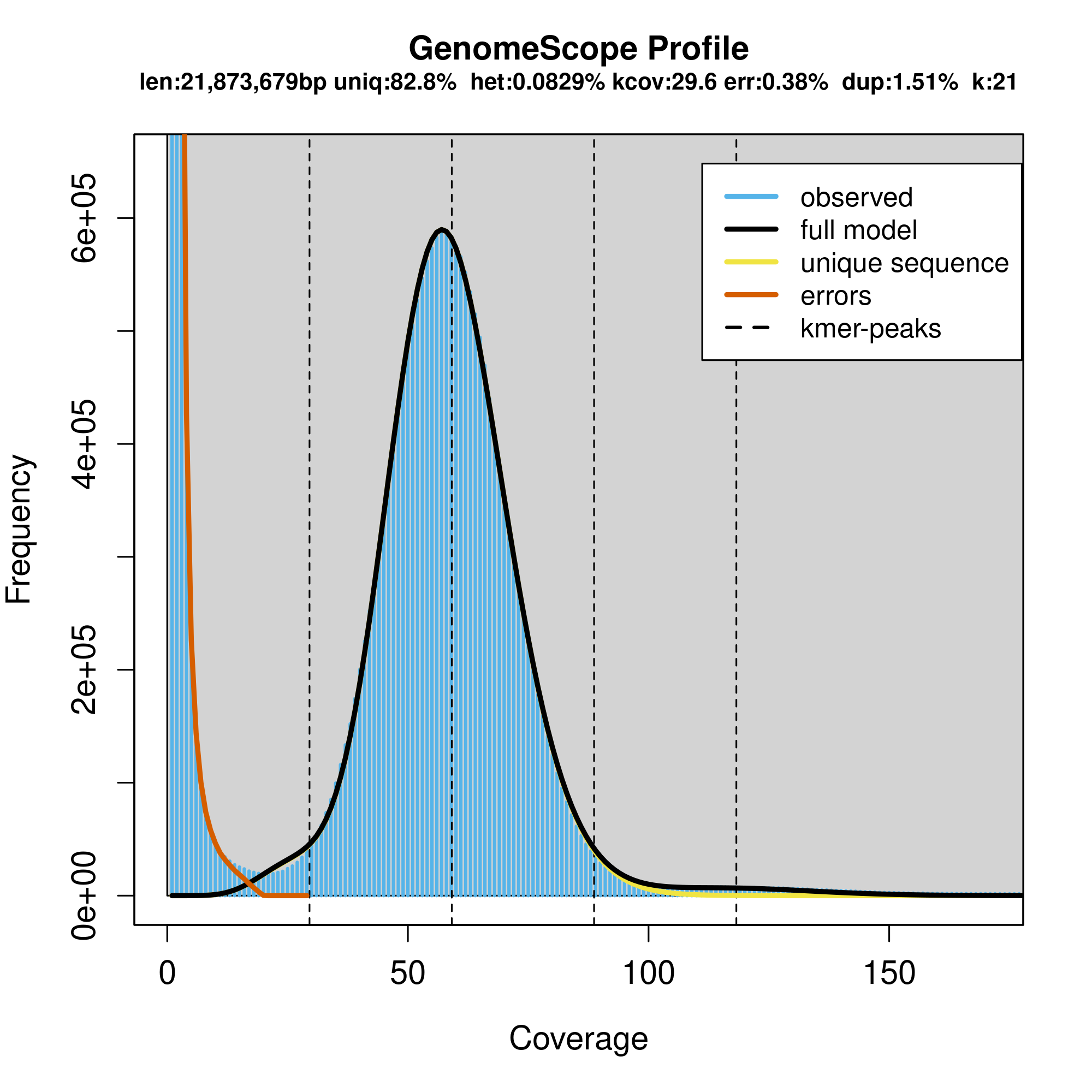
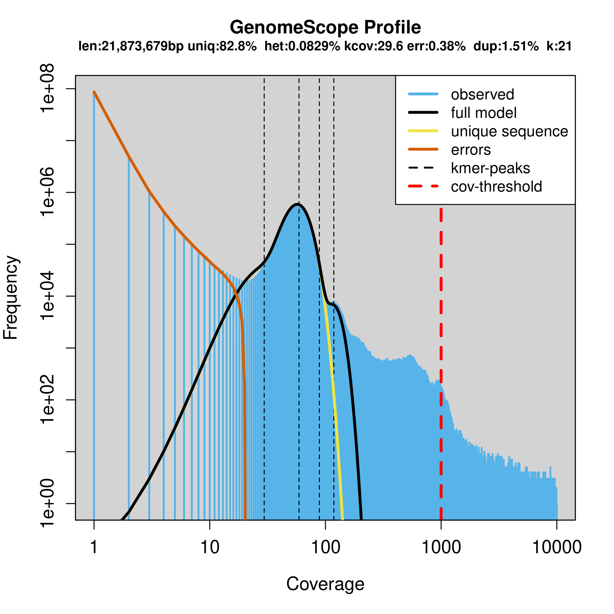
Common Elements in Both Figures

• Genome Size (len): Estimated genome size is 21,873,679 bp (~21 Mb).
• Unique Sequence (uniq): 82.8% of the genome is unique sequence.
• Heterozygosity (het): The heterozygosity rate is 0.0829%, indicating a very low level of heterozygosity.
• Coverage (kcov): Average k-mer coverage is 29.6.
• Error Rate (err): Estimated sequencing error rate is 0.38%.
• Duplication (dup): 1.51% of the genome is duplicated.
• k-mer size (k): k-mer length used for the analysis is 21.

Key Elements in the Plots

• X-Axis (Coverage): Represents the k-mer coverage. In the linear plot, it is shown on a linear scale, whereas in the logarithmic plot, it is shown on a logarithmic scale.
• Y-Axis (Frequency): Represents the frequency of k-mers at different coverage levels.
• Blue Bars (observed): Histogram of observed k-mer frequencies.
• Black Line (full model): Model fit to the observed k-mer frequencies.
• Yellow Line (unique sequence): Contribution of unique sequences to the k-mer frequencies.
• Orange Line (errors): Contribution of sequencing errors to the k-mer frequencies.
• Dashed Lines (kmer-peaks): Peaks corresponding to k-mer coverage of unique and repetitive sequences.
• Red Dashed Line (cov-threshold): A threshold to distinguish high-coverage k-mers, typically used to identify potential contaminant sequences or highly repetitive regions. This is set at a very high coverage level (around 1000).

Genome Assembly and Quality Assessment

This tutorial will guide you through the process of assembling a genome using HiFi reads and assessing its quality. We’ll be working with Arabidopsis thaliana chromosome 2 data as an example.

1. Genome Assembly with hifiasm

hifiasm is a fast and accurate haplotype-resolved assembler designed specifically for PacBio HiFi reads. It’s particularly effective because it can handle the high accuracy of HiFi reads while maintaining computational efficiency.

First, let’s create a directory for our assembly:

mkdir 06_Assembly 
module purge 
module load hifiasm 
time hifiasm -o 06_Assembly/chr2_hifi.asm -t 8 -m 10 01_Data/mapped_reads.chr2.filtlong.fastq.gz 
# Run hifiasm with the following parameters: 
# -o: output prefix 
# -t: number of threads (8 in this case) 
# -m: minimum number of overlaps to keep a contig (10 in this case) 

The assembly took approximately 3 minutes and 48 seconds to complete.

Converting Assembly Format from GFA to FASTA

The assembly output is in GFA (Graphical Fragment Assembly) format, which we need to convert to FASTA format for downstream analysis. GFA is a format that represents genome graphs, while FASTA is a more widely used format for sequence data.

# Extract sequences from GFA and convert to FASTA format 
awk '/^S/ { print ">"$2; print $3 }' 06_Assembly/chr2_hifi.asm.bp.p_ctg.gfa > 06_Assembly/chr2_hifi.asm.bp.p_ctg.fa 

Let’s check how many contigs we got from our assembly:

grep ">" -c 06_Assembly/chr2_hifi.asm.bp.p_ctg.fa 

Our assembly resulted in 63 contigs.

Assembly Statistics

./new_Assemblathon.pl 06_Assembly/chr2_hifi.asm.bp.p_ctg.fa > 06_Assembly/chr2_AssemblyStats.txt	 

less 06_Assembly/chr2_AssemblyStats.txt 

2. Quality Assessment

BUSCO Analysis with compleasm

BUSCO (Benchmarking Universal Single-Copy Orthologs) is a crucial tool for assessing genome assembly completeness. It searches for highly conserved genes that should be present in all species of a given lineage. The presence, absence, or fragmentation of these genes gives us insight into the quality of our assembly.

Key BUSCO metrics:

• Complete (S): Single-copy complete genes
• Duplicated (D): Complete genes present multiple times
• Fragmented (F): Partially assembled genes
• Missing (M): Genes not found in the assembly
• Total (N): Total number of genes in the BUSCO dataset

We’ll use compleasm, a faster implementation of BUSCO, with the embryophyta_odb12 database which is specific for plants:

module purge 
module load miniconda 
source activate /project/scinet_workshop2/Bioinformatics_series/Compleasm_conda/ 

time compleasm run -t 8 -l eukaryota -L 01_Data/busco/eukaryota_odb12 -a 06_Assembly/chr2_hifi.asm.bp.p_ctg.fa -o 07_Compleasm

This takes about 5 mins to run.

Understanding the BUSCO Results

Our assembly of chromosome 2 shows:

• 20.93% (27) complete single-copy genes
• 0.00% (0) duplicated genes
• 2.33% (3) fragmented genes
• 76.47% (99) missing genes
• Total: 129 genes assessed

These numbers are expected to be low since we’re only looking at one chromosome rather than the complete genome. For comparison, let’s look at the metrics for the complete Arabidopsis genome:

3. K-mer Based Quality Assessment

K-mer analysis is another powerful method for evaluating genome assembly quality. A k-mer is a substring of length k from a DNA sequence. By analyzing the distribution and frequency of k-mers in both our raw reads and assembly, we can assess assembly completeness and accuracy.

Step 1: Determining Optimal K-mer Size

First, we need to determine the optimal k-mer length for our analysis. This is important because:

• Too small k-mers may lead to random matches
• Too large k-mers may miss legitimate matches
• The optimal size depends on genome size and error rates

module purge 
module load merqury 
# Calculate optimal k-mer size based on genome size (19MB) 
best_k.sh 19000000 

Output:

 
genome: 19000000 
tolerable collision rate: 0.001 
17.0719 

The script suggests a k-mer size of 17 based on our genome size of 19Mb and a tolerable collision rate of 0.001.

Step 2: K-mer Analysis with Merqury

Merqury is a tool that evaluates genome assemblies using k-mer frequencies. It helps us understand:

• Assembly completeness
• Base-level accuracy
• Potential misassemblies

Let’s run the analysis:

# Count k-mers in the input reads 
time meryl k=17 count output 08_AT_HiFi.meryl 01_Data/mapped_reads.chr2.filtlong.fastq.gz 
# Create output directory and run Merqury 
mkdir 09_Merqury_Output_HiFi && cd 09_Merqury_Output_HiFi 
merqury.sh ../08_AT_HiFi.meryl \ 
  ../06_Assembly/chr2_hifi.asm.bp.p_ctg.fa merqury_out 

Step 3: Interpreting Merqury Results

Quality Value (QV) Statistics

Let’s examine the assembly quality values:

cat merqury_out.qv 

 
chr2_hifi.asm.bp.p_ctg  40      28858272        70.8866 8.15344e-08 

These metrics tell us:

• Assembly Name: chr2_hifi.asm.bp.p_ctg
• Unique K-mers: 40 k-mers found only in the assembly
• Total K-mers: 28,858,272 k-mers found in both assembly and reads
• Quality Value (QV): 70.89 - this is excellent! QV is a logarithmic measure of error probability
• Error Rate: 8.15e-08 - extremely low, indicating very high accuracy

Completeness Assessment

Let’s check the assembly completeness:

cat merqury_out.completeness.stats 

 
chr2_hifi.asm.bp.p_ctg  all     18214072        18235904        99.8803 

These statistics show:

• Covered Bases: 18,214,072 bases are supported by k-mers from our input reads
• Total Bases: 18,235,904 bases in our assembly
• Completeness: 99.88% - this is exceptional! It means almost every base in our assembly is supported by the input reads

Exercises

1. Download the saccharmycetes busco lineage and run compleasm on the yeast genome assembly in 00_Miscellaneous_Data/yeast.fasta
   Hint: check compleasm download -h

2. Use the yeast nanopore reads 00_Miscellaneous_Data/SRR18210286_filtlong_500Mb.fastq.gz to get the merqury qv of the yeast genome assembly 00_Miscellaneous_Data/yeast.fasta.
   Hint: The genome size of yeast is approximately 12 MB.

• • Tuesday, April 29, 2025, 1 – 5 PM ET
    • Prerequisites:
      • Familiarity with basic command-line concepts.
    • Workshop recording