
In this workshop, participants will work through a complete RNA-seq analysis using SCINet’s Galaxy interface. Participants will learn how to create workflows in Galaxy to:
- Upload and process RNA-seq data.
- Perform quality control, alignment, and expression quantification.
- Identify differentially expressed genes using DESeq2.
We will also explore ways in which you can share your history and workflows with other SCINet users in Galaxy and how it can be a powerful tool for collaborations.
At this time, registration is closed as we have reached maximum capacity for all workshops. However, you may complete the registration form to be added to our waitlist for future offerings.
Pre-Workshop Instructions:
To help minimize technical issues and delays at the start of the workshop, please try the following tests prior to the workshop.
- Logging on to Ceres Open OnDemand (OOD):
- Please confirm you can successfully log in to Ceres OOD with your SCINet account (see OOD login instructions here). If you are successful, you will be able to see the Ceres OOD home page.
- Ceres Shell Access:
- When on Ceres OOD, click on the top navigation bar: “Clusters” > “Ceres Shell Access”. A new tab will appear that looks like a shell terminal (e.g., like PowerShell).
- Please confirm you do not receive any error messages or requests to re-authenticate and that the final line looks like “[firstname.lastname@ceres ~]$”.
- Logging on to Galaxy:
- Please confirm you can successfully log in to Galaxy on SCINet with your SCINet account (see Galaxy login instructions here). If you are successful, you will be able to see the standard Galaxy home screen.
- Importing data to Galaxy
-
While on Ceres Shell Access, navigate to your Galaxy folder in your home directory on Ceres
cd /home/$USER/galaxy -
Copy workshop data to your Galaxy folder on Ceres by copying the commands below and running them in the Ceres terminal.
cp /90daydata/shared/galaxy_workshop/GCF_000001735.4_TAIR10.1_genomic.fna . cp /90daydata/shared/galaxy_workshop/GCF_000001735.4_TAIR10.1_genomic.gtf . cp /90daydata/shared/galaxy_workshop/*.gz . - After copying the files to your Galaxy folder, return to the Galaxy tab in your web browser. (If you are not already logged on to Galaxy, please see “Logging on to Galaxy”, above.)
- You will import files into Galaxy by clicking on “Upload” in the left panel of the Galaxy home screen. The following download/upload screen should appear:
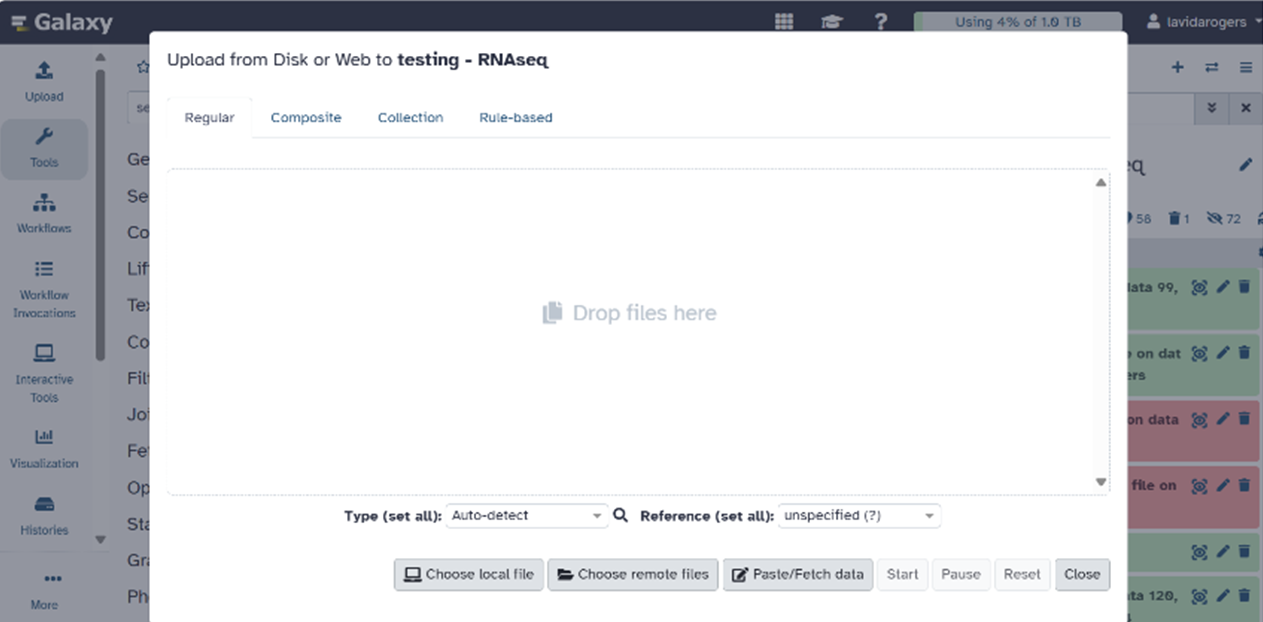
- Click on “Choose remote files.” This will show you the files in your Galaxy folder on Ceres.

- Select the files you want to transfer.
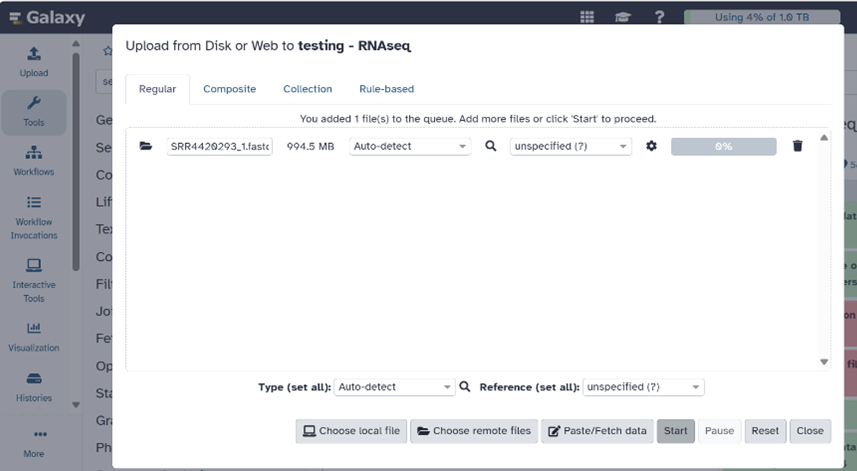
- Click “Start” and wait for the files to be imported into Galaxy. The files will appear in the History pane on the right of your home screen.
-
For more information on importing data to Galaxy, see the SCINet Galaxy user guide.
RNA-Seq Data Analysis with Galaxy
by Siva Chudalayandi and Lavida Rogers
RNA-seq experiments are designed to comprehend transcriptomic changes in organisms in response to a certain treatment. They are also designed to understand the cause and/or effect of a mutation by measuring the resulting gene expression changes. Robust algorithms specifically designed to map short stretches of nucleotide sequences to a genome while being aware of the process of RNA splicing have led to many advances in RNAseq analysis. An overview of RNA-seq analysis is summarized in Figure 1.

This tutorial will guide you through a basic RNAseq analysis with Galaxy, beginning at quality checking of the RNA-seq reads through to differential gene expression analysis. We will complete the following tasks:
- Quality Control
- Read alignment
- Abundance estimation
- Differential gene expression analysis
- Visualization and biological interpretation
We have downloaded an Arabidopsis dataset from NCBI for this purpose. Check the BioProject page for more information.
Background Information: Experimental design
This experiment compares wild type (WT) and atrx-1 mutant Arabidopsis to analyze how the loss of function of ATRX protein results in changes in gene expression. The ATRX protein is a histone chaperone known to be an important player in the regulation of gene expression. RNA was isolated from three WT replicates and three mutant replicates. The transcriptome was enriched/isolated using the plant RiboMinus kit for obtaining total RNA. RNA-seq was carried out on Illumina Hiseq 2500. The sequencing reads are paired-end data, hence we have 2 files per replicate.
| Condition | replicate 1 | replicate 2 | replicate 3 |
|---|---|---|---|
|
WT |
SRR4420293_1.fastq.gz |
SRR4420294_1.fastq.gz |
SRR4420295_1.fastq.gz |
|
atrx-1 |
SRR4420296_1.fastq.gz |
SRR4420297_1.fastq.gz |
SRR4420298_1.fastq.gz |
Preparation
If you missed the pre-workshop help session, see the pre-workshop instructions to get started with using Galaxy on SCINet.
Setting up your workspace
When you login to Galaxy, your History panel will be empty or contain previous work (if you attended the pre-workshop help session or have used Galaxy before). The Galaxy history is a workspace that stores data, tool outputs, and intermediate results so your work can be reviewed, shared, or rerun at anytime.
We will begin by creating a new history:
- Locate the history panel on the right side of the Galaxy interface, click the
+to create a new history. - Click the history title (default: Unnamed history)
- Rename the history to
RNA-seq_QCandLogs - Save changes


We will use this history for quality control and preprocessing.
Importing data to Galaxy
Data can be uploaded to Galaxy from a local machine, from remote sources (URLs and Ceres Galaxy folder), or from a shared history.
Instructions to upload data to Galaxy via Ceres can be found in the pre-workshop instructions.
For this workshop, we will import data via a shared Galaxy history that we created prior to the workshop. Here is the link to a Galaxy history with all the files needed for the workshop.
Sharing data via histories is also a great option for working with collaborators.
After clicking the shared history link, you will see “Import this History.” Click on it to import the files. Galaxy imports shared histories as new histories. This new history will now contain 12 FASTQ files, the Arabidopsis genome (.fa), the annotation file (.gtf), and a gene categories file (.txt).

Let’s rename the imported history to RNA-seq_analysis.

Why are we working with two histories? Galaxy does not allow histories to be merged. Instead, datasets can be copied between histories as needed as we move through workflows. Using multiple histories helps keep our main analysis and quality control, logs, and preprocessing steps separate.
Job statuses in Galaxy
To understand the stages of your jobs as we progress through the tutorials, you will need to understand how Galaxy displays job statuses.
- Grey: The job is queued.
- Yellow: The job is running.
- Green: The job has completed successfully.
- Red: The job has failed.
- Light Blue: The job is paused.
Now that we know what job status is represented by each color used in Galaxy, we can get started!
Preparing the data for downstream analysis
While still in the RNA-seq_analysis history, we will start by organizing our sequencing data so that read pairing is preserved and sample identity (mutant vs wildtype) is clear.
This preparation involves renaming the datasets, creating paired dataset lists, and flattening collections as needed.
-
Renaming datasets in Galaxy
First, we’ll rename the data files so that it is easier to see which files represent mutant or WT samples.
- In the history panel, locate the 12 FASTQ datasets.
- Click on the pencil icon to edit attributes of
SRR4420293_1.fastq.gzand rename this file toWT_SRR4420293_1 - Save changes.
-
Rename the remaining files as follows:
Original File Name New Name SRR4420293_2.fastq.gz WT_SRR4420293_2.fastq.gz SRR4420294_1.fastq.gz WT_SRR4420294_1.fastq.gz SRR4420294_2.fastq.gz WT_SRR4420294_2.fastq.gz SRR4420295_1.fastq.gz WT_SRR4420295_1.fastq.gz SRR4420295_2.fastq.gz WT_SRR4420295_2.fastq.gz SRR4420296_1.fastq.gz MUT_SRR4420296_1.fastq.gz SRR4420296_2.fastq.gz MUT_SRR4420296_2.fastq.gz SRR4420297_1.fastq.gz MUT_SRR4420297_1.fastq.gz SRR4420297_2.fastq.gz MUT_SRR4420297_2.fastq.gz SRR4420298_1.fastq.gz MUT_SRR4420298_1.fastq.gz SRR4420298_2.fastq.gz MUT_SRR4420298_2.fastq.gz
-
Create Paired Dataset Lists
The data we are working with are paired-end sequencing reads, so we will create paired dataset lists. Paired lists preserve the relationship between forward and reverse reads. Galaxy automatically detects paired reads based on file name patterns.
Commmon pairing patterns:
- _R1 and _R2
- _1 and _2
Steps for creating paired dataset lists:
- In the history panel, click marked check box to enable file selection.
- Select the WT FASTQ files.
- Click on the down arrow that appears near
6 of 14 selectedand select advanced build list. - Select list of paired datasets.
- Based on the filenames having common pairing patterns, Galaxy will autopair.
- Save this list as
ATRX_wildtype. - Next, we will repeat the above steps for the MUT files and save the list as
ATRX_mutant.
-
Flatten Paired Lists
Some tools such as FASTQC and MultiQC do not require nested pairing structure. Flattening will produce one dataset per sample and ensure forward and reverse reads are not treated separately.
Here we will create a flattened collection to simplify the QC steps:
- Search for the tool: Flatten Collection.
- Select the collections you want to flatten:
ATRX_wildtype. - Run the tool.
- Rename the output:
ATRX_wildtype_flattened. - Repeat the above steps to also flatten the mutant dataset collection.
-
Move flattened collections
At this point, paired datasets have been created and flattened. We will now moves these flattened collections into the QC history we created at the beginning of the tutorial.
To make copying easier, Galaxy allows you to view two histories at once, side-by-side.
Steps:- Open the History panel.
- Click the History options menu (three lines).
- Select Show histories side by side.

- Choose:
- Left:
RNA-seq_analysis - Right:
RNA_seq_QCandLogs
You should now see both histories.
- Left:
- Drag and drop the two flattened lists to the
RNA_seq_QCandLogs. - Switch to the
RNA_seq_QCandLogshistory.
Quality Control
We use FastQC, a tool that provides a simple way to do quality control checks on raw sequence data coming from high-throughput sequencing pipelines.
-
FastQC
- Go to the Tools panel and search for
FastQC. - Set the parameters for FastQC:
- Input files: Raw read data from your current history
- Select a flattened collection:
ATRX_wildtype_flattened - Leave all other parameters at their default settings.
- Run the tool.
- To view output, click the eye icon on the fastqc output.
- Repeat for
ATRX_mutant_flattened.
- Go to the Tools panel and search for
-
MultiQC
After running fastqc on multiple datsets, we can use MultiQC to combine all QC reports into a single summary report. This allows you to produce a report that compares results from all samples.
- Go to the tools panel and search for multiQC.
- Which tool was used generate logs? Select FASTQC.
- Type of FastQC output: Raw Data
- Select the relevant collections (both WT and mutant)
- Run the tool.
- Both HTML and Stats outputs are produced.
You can preview the HTML output in Galaxy and inspect for any problems.
-
Trimming
We will use Trim Galore to trim adapters off the RNAseq reads. This is a wrapper script around
cutadapt.- Go to the Tools Panel and search for Trim galore.
- Parameters:
- Library: paired-end collection
- Adapter sequence: Automatic detection
- Settings: Default
- Run the tool.
- Output: Trimmed Collection for each input.
-
Transition to RNA-seq Analysis History
At this point, reads are analysis-ready.
Next, we will copy the trimmed FASTQ files into the
RNA_seq_analysishistory and switch histories.The
RNA_seq_analysishistory should now contain your trimmed FASTQ files, the reference genome, and the GTF annotation file.Note: Galaxy does not overwrite data. Every action creates a new dataset, so your original files remain unchanged.
Mapping to a reference genome
There are several mapping programs available for aligning RNAseq reads to the genome. Generic aligners such as BWA, bowtie2, BBMap, etc., are not suitable for mapping RNAseq reads because they are not splice-aware. RNAseq reads are mRNA reads that only contain exonic regions, hence mapping them back to the genome requires splitting the individual reads that span an intron. It can be done only by splice-aware mappers.
In this tutorial, we will use HISAT2, a successor of Tophat2.
Steps for using HISAT2 in Galaxy:
- Search the tool panel for HISAT2.
- Set your parameters:
- Source for reference genome: Use a genome from history
- Is this a single or paired library: Paired-end dataset collection (because we created a collected of the raw fastq files)
- Galaxy tries to automate the steps as much as possible, so because you indicated that the library is a paired-end dataset collection, Galaxy automatically selected the collection in your history.
- Paired collection: raw files (a collection in your history)
- Note to always double check selected inputs even if Galaxy automatically selects the accepted formats.
- Specify strand information * reverse (RF)
- All other parameters can remain set to default settings.
- Run the tool.
Abundance Estimation
For quantifying transcript abundance from RNA-seq data, there are many programs available. Popular tools include featureCounts and HTSeq. We will need a file with aligned sequencing reads (SAM/BAM files generated in previous step) and a list of genomic features (from the GFF file).
featureCounts is a highly efficient general-purpose read summarization program that counts mapped reads for genomic features such as genes, exons, promoter, gene bodies, genomic bins and chromosomal locations. It also outputs statistics for the overall summarization results, including the number of successfully assigned reads and the number of reads that failed to be assigned due to various reasons. We can run featureCounts on all SAM/BAM files at the same time or individually.
Steps for running featureCounts in Galaxy:
- Search for the tool featurecounts.
- Set the parameters:
- Alignment file : dataset collection
- Specify strand information * RF
- Gene annotation file: A GFF/GTF file in your history - automatically selects the annotation file, but always double check.
- Does the input have read pairs? Yes, paired end, but count them as a single fragment
- Run the tool.
Differential Gene Expression Analysis
After read alignment and read counting, differental expression analysis is performed with DESeq2. This identifies genes whose expression differ significantly between factors (mutant vs. wildtype samples)
DESeq2 normalizes count data, estimates dispersion across replicates, and tests for differential expression between defined conditions. In Galaxy, we will use the tool DESeq2 and manually assign samples to experimental conditions.
- Search for Deseq2 in the tool panel.
- Set the tool parameters:
- How: select datasets per level
- Factor Name: genotype
- Factor Level: wildtype
- Count files:
- Factor Level: mutant
- Count files:
- Leave others to default settings
- Run the tool.
Functional interpretation and reproducible workflows in Galaxy
Functional enrichment with GOseq
We have identified differentially expressed genes and now we want to biologically interpret what these results mean. Biological interpretation requires asking:
Are there any biolgical functions or processes that are overrepresented among these genes?
Gene ontology (GO) enrichment analysis helps us answer this question by testing whether genes associated with specific biological processes (BP), molecular functions (MF), or cellular components (CC) occur more frequently than expected by chance.
GOseq is an R-based method designed for handling RNA-seq data. GOseq works by modeling the relationship between gene length and differential gene expression and adjusting enrichment tests to account for biases (count and gene length biases). GOseq is an R package and in this case, Galaxy will execute R code through the tool GOSeq in the background and return the results as Galaxy datasets.
Attribution: The following steps in this tutorial were adapted from the Galaxy Training Network Reference-based RNA-seq tutorial with modifications for this workshop.
Prepare inputs for GOSeq
To run GOSeq, we need three inputs:
- Differential gene expression results
- Gene length information
- Gene category mapping (GO terms) (imported from the shared history)
-
Prepare the first input for GOseq
The purpose of this step is to convert the DESeq2 results table into a binary indicator identifying whether each gene is differentially expressed. In this step we will be generating a boolean (TRUE/FALSE) variable based on the adjusted p-value threshold
(p<0.05).Steps:
- Search for the tool “Compute on rows” in the tool panel.
- Set the following parameters:
- Input file: the DESeq2 result file
- Add expression: bool(float(c7)<0.05)
- c7: column 7 (adjusted p-value)
- float(c7): allows numeric comparisons
- <0.05: the significant threshold
- bool(…): converts to True/False*
- Mode of the operation: Append
- Under “Error handling”:
- Autodetect column types: No
- If an expression cannot be computed for a row: Fill in a replacement value
- Replacement value: False
- Run the tool.
This creates an additional column in the DESeq2 results table that indicates if a gene is differentially expressed. GOSeq only needs the gene names and the binary indicator, so next we will generate a new dataset with only these two columns.
Steps:
- Search for the tool “Cut”.
- Set parameters:
- Cut columns: c1,c8
- Delimited by: Tab
- From: the output of the Compute tool
- Run the tool.
To ensure all gene names are capitalized, we will have Galaxy change the case of the gene name column:
- Search for the tool “Change Case”.
- Set parameters:
- From: the output of the previous Cut tool
- Change case of columns: c1 (first column with gene names)
- Delimited by: Tab
- To: Upper case
- Run the tool.
- Rename the output to “Gene IDs and differential expression”.
-
Prepare the gene length file
We will now extract the gene length information.
Steps:
- Search for the tool “Extract Dataset”.
- Set parameters:
- Input List: featureCounts on collection N: Feature lengths
- How should a dataset be selected?: The first dataset
- Run the tool.
Change Case of the above output with the following parameters:
- Search for the tool “Change Case”.
- Set parameters:
- From: output of Extract Dataset tool
- Change case of columns: c1
- Delimited by: Tab
- To: Upper case
- Rename the output to “Gene IDs and length”.
-
Running GOSeq
Steps:
- Search for the “GOSeq” tool.
- Set the parameters:
- Differentially expressed genes file: Gene IDs and differential expression
- Gene lengths file: Gene IDs and length
- Gene categories: Use a category file from history
- Gene category file: GO categories
- Output Options:
- Output Top GO terms plot?: Yes
- Extract the DE genes for the categories (GO/KEGG terms)?: Yes
- Run the tool.
GOSeq outputs include:
-
A table (Ranked category list - Wallenius method) with the following columns for each GO term:
Column Definition category GO category over_rep_pval p-value for under-representation of the term in DE genes under_rep_pval p-value for over-representation of the term in DE genes numDEInCat number of DE genes in category term term details ontology MF (Molecular Function),
CC (Cellular Component),
BP (Biological Process)p.adjust.over_represented p-value for over-representation of the term in DE genes, adjusted for multiple testing p.adjust.under_represented p-value for under-representation of the term in DE genes, adjusted for multiple testing - A graph with the top 10 over-represented GO terms.
- A table with the differentially expressed genes (from the list we provided) associated to the GO terms (DE genes for categories (GO/KEGG terms)).
Introduction to Galaxy workflows
Once an RNA-seq analysis is complete and the results make biological sense, the next critical step is to capture how we got to the final results. In Galaxy, a user can build a workflow directly from their history, which transforms a series of interactive steps into a structured, reusable analysis pipeline. This workflow provides a clear big-picture view of the entire RNA-seq process, from raw reads to differential expression.
The workflow can be edited to reflect the decisions made during the analysis (such as alignment options, or statistical thresholds), creating a structured framework for automation, reproducibility, and error checking. Once finalized, the workflow can be run end-to-end on new datasets and shared with collaborators, allowing analyses to be reproduced, reviewed, and adapted with transparency.
In this section, we will go step by step through the process of creating a Galaxy workflow. Specifically, we will show how to create a workflow for our analysis of RNA-seq data from Arabidopsis mutant and wild-type (WT) samples.
We followed a standard RNA-seq strategy:
- Align reads to a reference genome
- Count reads per gene
- Statistically compare gene counts between conditions
Galaxy allows us to do this reproducibly using a workflow. Before we create the workflow, let’s walk through the main steps our workflow will include.
-
What are the inputs to the workflow?
It’s critical to understand the inputs.
Everything else in the workflow is a transformation of these four inputs.Input Description Why it matters Genome (FASTA)
Arabidopsis reference genome
reads are aligned to this
GTF annotation
Gene and exon definitions
Needed for counting reads per gene
Mutant reads
Paired-end RNA-seq reads (collection)
Condition 1
WT reads
Paired-end RNA-seq reads (collection)
Condition 2
Key idea:
The genome and GTF are shared, but the reads represent biologically independent conditions. -
One workflow, two analyses
This workflow is best understood as two sub pipelines.
Conceptually:
     Genome + GTF
           |
-----------------------
|                     |
Mutant reads       WT reads
|                     |
HISAT2            HISAT2
|                     |
featureCounts     featureCounts
 \                   /
       DESeq2
Galaxy makes this explicit by running the same tools twice (seemingly in parallel). Mutant and WT samples are processed independently until they are compared statistically during differential expression analysis.
-
HISAT2: aligning RNA-seq reads
HISAT2 is run twice:
- Once for the mutant read collection
- Once for the WT read collection
Both use:
- The same genome
- The same GTF annotation
Output:
- BAM files containing aligned reads
Important point: Duplicated tools in Galaxy workflows represent explicit data flow, not redundant analysis.
-
featureCounts: from reads to genes
From this point onward, RNA-seq data analysis becomes a gene-level counting problem.
featureCounts:
- Uses the GTF to define features/genes
- Assigns aligned reads to genes
- Produces one count table per condition
Output:
- Mutant gene count table
- WT gene count table
Each row corresponds to a gene. Each column corresponds to a sample.
-
DESeq2: statistical comparison
DESeq2:
- Takes gene count tables
- Models biological variability
- Tests for differential expression
Output includes:
- log2 fold change
- p-value
- adjusted p-value (FDR)
Key idea: DESeq2 operates on counts only, not on alignments or reads.
-
What this workflow does NOT include
This workflow only focuses on core analysis and excludes:
- Read-level QC (FastQC, MultiQC)
- Alignment QC (flagstat, MultiQC)
- Functional interpretation (GO or KEGG)
These steps are intentionally excluded from the workflow because:
- QC is often iterative and exploratory. Including QC in a fixed workflow can obscure judgment calls.
- GOseq (Functional interpretation) is omitted because it is context-dependent and better dealt with separately.
- We have tried to preserve both analytical rigor and conceptual clarity for the purpose of this workshop.
NOTE: At this stage, we have a complete RNA-seq analysis that produces biologically interpretable results. However, the analysis exists only as a sequence of interactive steps in a Galaxy history. While this is ideal for exploration and learning, it becomes a liability when we want to repeat the analysis, apply it to new data, or share it with others. Converting it to a Galaxy workflow makes it ready for sharing and re-use.
Editing and sharing the Galaxy workflow
Up to this point, we have focused on running the analysis. As we’ve discussed, a Galaxy workflow will make our analysis reusable and shareable, so let’s create a new workflow now!
-
Extracting a workflow from a history
Any completed analysis history can be converted into a workflow:
- Open the history menu
- Select Extract Workflow
- Choose the steps to include
- Save the workflow
This allows exploratory analyses to be turned into structured, reusable pipelines.
-
Editing the workflow
A workflow can be edited at any time:
- Open the workflow menu
- Select Edit
- Modify tool parameters, inputs, or connections
- Save the updated workflow
Edits do not affect previously run histories. Each workflow version represents a reproducible analysis state.
Typical reasons to edit a workflow include:
- Changing reference genome or annotation
- Adjusting tool parameters
- Adding or removing analysis steps
- Adapting the workflow for a different experiment
-
Sharing workflows
Workflows can be shared with collaborators or the broader community:
- Shared via direct link
- Published within a Galaxy instance
- Exported as a workflow file for use on other Galaxy servers
Sharing a workflow allows others to:
- Reproduce the analysis
- Inspect all parameters
- Run the same analysis on the new data


Conclusions
Galaxy workflows are not just automation tools. They function as:
- Analysis documentation (complete with help and readme)
- Reproducible methods
- Shareable computational protocols
Once a workflow is shared, the analysis becomes transparent, repeatable, and extensible.